Motivation

• Heteregeneous Autoregressive model is now over 15 years old.
• Well-established interpretable benchmark for realized volatility (RV) forecasting.
• Today, machine learning (ML) methods are at the center of nearly all modern research, seemingly surpassing HAR in many scenarios .

Our Contribution

• Demonstrate that seemingly minor modeling choices may drastically impact HAR's performance.
• Review previous works where ML outperforms HAR with and put these results into perspective.
• Study an unprecedented dataset of 1,455 U.S. stocks.
• Suggest ideal estimation approach for the HAR model.

Data

• High-frequency intraday data from Trades and Quotes (TAQ).
• 6,061 U.S. stocks the Center for Research in Security Prices (CRSP).
• ~9 years: January 1, 2015, to October 31, 2023.
• 1,455 stocks are consistently traded throughout the 9-year period.
• 27 / 30 of the Dow Jones Industrial Average (DJIA).
• 69 / 100 of the Nasdaq-100.

HAR Model

$$\mathrm{RV}_{i,t+1}^{(d)} = c + \beta^{(d)} \mathrm{RV}_{i,t}^{(d)} + \beta^{(w)}\mathrm{RV}_{i,t}^{(w)} + \beta^{(m)}\mathrm{RV}^{(m)}_{i,t} + \epsilon_{i,t+1},$$ where $\mathrm{RV}_{i,t}^{(d)}$ denotes the logarithm of the daily realized volatility of stock $i$ at time $t$ and

• $\mathrm{RV}_{i,t}^{(w)} = \frac{1}{5}\sum_{h=1}^5 \mathrm{RV}_{i,t-h+1}^{(d)}$
• $\mathrm{RV}_{i,t}^{(m)} = \frac{1}{22}\sum_{h=1}^{22} \mathrm{RV}_{i,t-h+1}^{(d)}$

HAR Model

$$\mathrm{RV}_{i,t+1}^{(d)} = c + \beta^{(d)} \mathrm{RV}_{i,t}^{(d)} + \beta^{(w)}\mathrm{RV}_{i,t}^{(w)} + \beta^{(m)}\mathrm{RV}^{(m)}_{i,t} + \epsilon_{i,t+1},$$ where $\mathrm{RV}_{i,t}^{(d)}$ denotes the logarithm of the daily realized volatility of stock $i$ at time $t$ and

• $\mathrm{RV}_{i,t}^{(w)} = \frac{1}{5}\sum_{h=1}^5 \mathrm{RV}_{i,t-h+1}^{(d)}$
• $\mathrm{RV}_{i,t}^{(m)} = \frac{1}{22}\sum_{h=1}^{22} \mathrm{RV}_{i,t-h+1}^{(d)}$

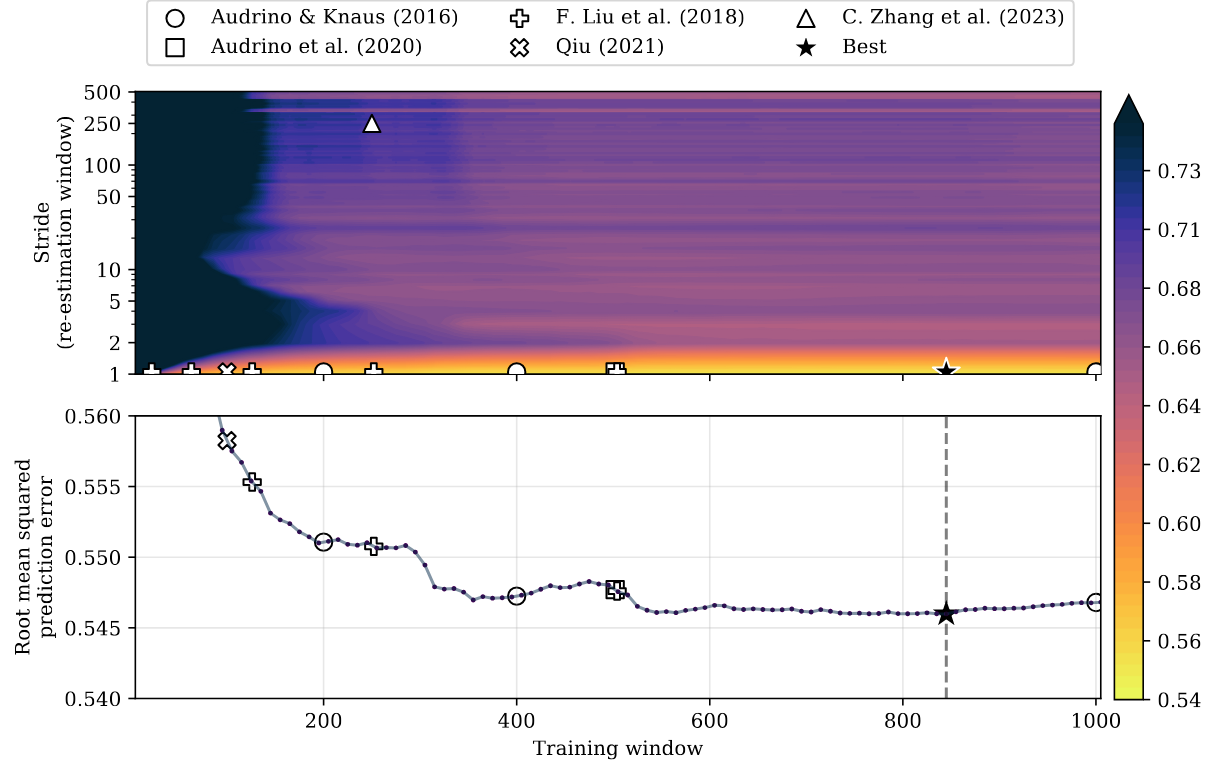
Estimating the Coefficients

Typically, HAR is estimated in a rolling or expanding fashion, i.e., a researcher must choose:

• how often to re-fit the model (stride or re-estimation frequency/window)
• on how much data to fit the model (training window)
• whether to roll or expand the training data

Current Studies

Models

HAR model

• Estimate via OLS and WLS
• Estimate individually and in a pooled manner

ML models

• Lasso
• Random Forest
• Gradient Boosted Trees
• Feedforward Neural Networks

Comparison

• Mean Squared Error (MSE), QLIKE , and Realized Utility .
• Each model is estimated once using only past RVs and once with the addition of the VIX (16 models).
• Compare distributions of the losses.
• For every asset, compute the model confidence set with a 95% level of confidence.
• Repeat the comparison for the DJIA and Nasdaq-100 universes only.

Conclusion

• A properly fitted HAR model still reigns supreme for RV forecasting.
• Use a properly fitted HAR model as benchmark when comparing your novel method…
• estimate in a rolling manner,
• re-estimate daily,
• use between 2.5 and 4 years of training data
• estimate via weighted least squares,

References