Introduction to Machine Learning
Workshop Fundamentals of Data Science
Jonathan Chassot
October 30, 2023
What is machine learning?
What is machine learning?
- Nature
- Not a single approach but a wide array of techniques
- Foundations
- Probability theory, Statistics, Linear algebra, Optimization, Control theory
- Applications
- Classification, Regression, Clustering, Density estimation, …
- Related Fields
- Probability theory, Statistical inference, Computational statistics, Data mining, Data science, Computer vision, Artificial intelligence, optimization theory, …
What is machine learning?
- Pattern recognition
- Identifying and understanding patterns in the data
- Improvement over time
- Systems perform better as more data becomes available
- Less manual interventions required as they learn
- Data-driven decisions
- Making decision based on analyzed data rather than pre-defined rules
- Generalization
- Applying learned knowledge to unseen data or scenarios
- Not just memorizing but understanding patterns
- Adaptation
- Changing behavior in response to changing environments or data trends
Main Types of Learning
- Supervised Learning
- Unsupervised Learning
- Reinforcement Learning
- Self-supervised Learning
Main Types of Learning
- Supervised Learning
- Use labeled data to learn how to make predictions.
- E.g., predicting tomorrow's stock price, predicting the number of sales in a particular month
- Unsupervised Learning
- Use unlabeled data to discover patterns
- E.g., clustering similar type of films or songs
- Reinforcement Learning
- Learning through trial and error to maximize rewards
- E.g., self-driving cars, stock-trading bots
- Self-supervised Learning
- Use its own modified data as a label
- E.g., language models, generative models

This course will focus on supervised learning, where our machine is being supervised by labeled data. Like teaching a child with examples; every piece of data comes with a correct answer.
Definition
A computer program is said to learn from experience $E$ with respect to some class of tasks $T$ and performance measure $P$, if its performance at tasks in $T$, as measured by $P$, improves with experience $E$. (Mitchell, 1997)
Definition
A computer program is said to learn from experience $E$ with respect to some class of tasks $T$ and performance measure $P$, if its performance at tasks in $T$, as measured by $P$, improves with experience $E$. (Mitchell, 1997)
Three ingredients:
- Experience $E$
- Class of tasks $T$
- Performance $P$
Definition
- Experience $E$
- $\mathcal{X}$ - input space (measurement space, feature space)
- $\mathcal{Y}$ - output space (label space, response space)
- Class of tasks $T$
- determine a true function $f : \mathcal{X} \to \mathcal{Y}$
- Performance $P$
- reward or utility function (its negative is a loss function)
Examples
- Experience $E$
- $\mathcal{X}$ - temperature, season, sunshine duration
- $\mathcal{Y}$ - number of bikes rented
- Class of tasks $T$
- determine a function which takes as input the temperature, the season, and sunshine duration to predict the number of bikes rented
- Performance $P$
- …?

Examples
- Experience $E$
- $\mathcal{X}$ - market news, analyst ratings, past price
- $\mathcal{Y}$ - future stock price
- Class of tasks $T$
- determine a function which takes as input market news, analyst ratings, and past stock prices to predict future stock prices
- Performance $P$
- …?

Examples
- Experience $E$
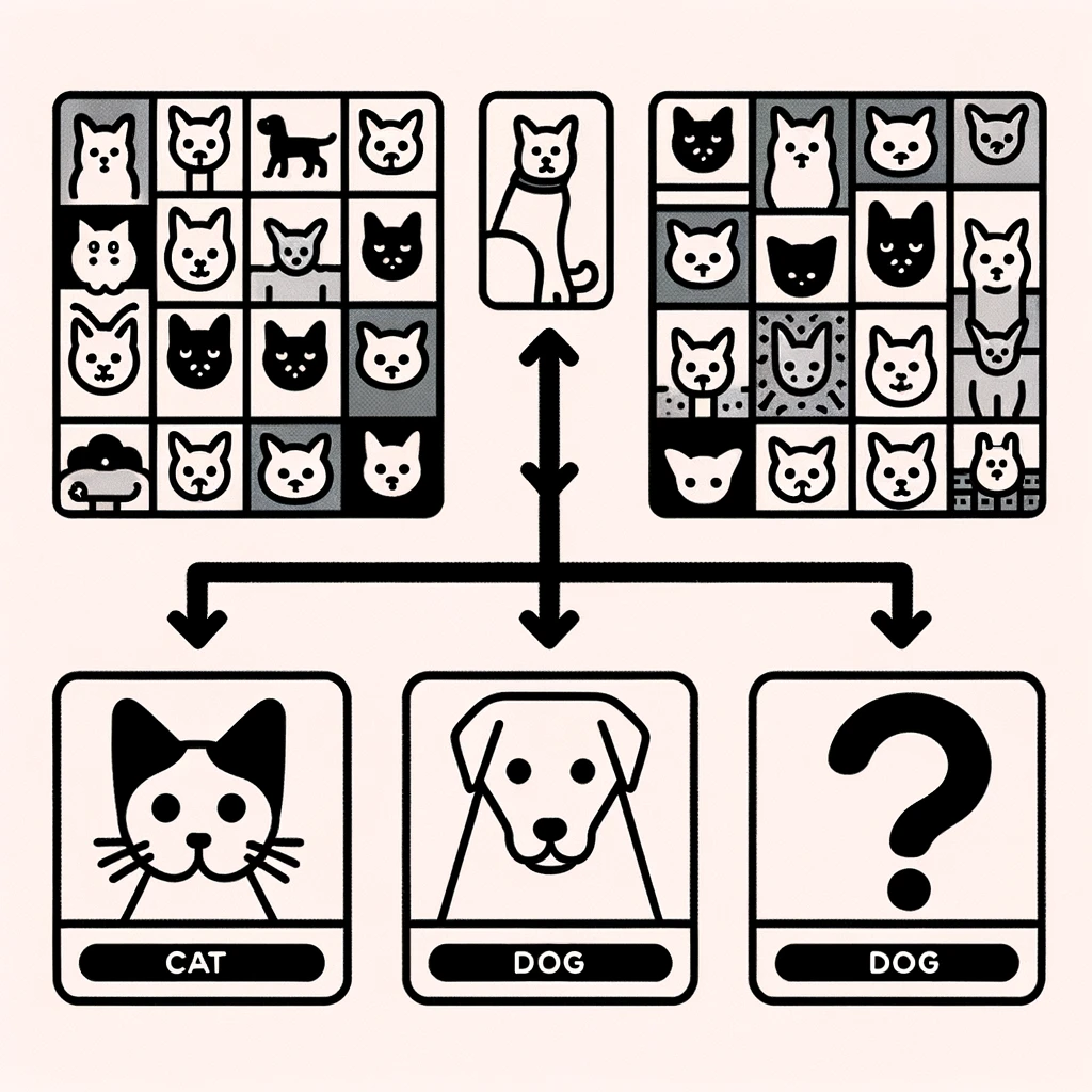
- $\mathcal{X}$ - images of dogs or cats
- $\mathcal{Y}$ - "dog" or "cat"
- Class of tasks $T$
- determine a function which takes an image as input and assesses whether the image is of a cat or a dog
- Performance $P$
- …?

Experience
In supervised learning, experience is straightforward: a dataset of features and matching labels, e.g.,
- $\mathcal{X}$ - temperature, season, sunshine duration
- $\mathcal{Y}$ - number of bikes rented
- $\mathcal{X}$ - market news, analyst ratings, past price
- $\mathcal{Y}$ - future stock price
- $\mathcal{X}$ - images of dogs or cats
- $\mathcal{Y}$ - "dog" or "cat"
Classes of tasks $T$
Do the following examples belong to the same class of tasks?
- Assessing if an image is of a cat or a dog
- Predicting the number of bike sales
- Predicting future stock prices
- Predicting whether the price of stock is going to go up or down
- Predicting whether a creditor will default
- Predicting the number of passengers in a given flight
- Predicting the age of a viewer of an online video
Classes of tasks $T$
- Regression
- Predicting future stock prices
- Predicting the number of bike sales
- Predicting the age of a viewer of an online video
- Predicting the number of passengers in a given flight
- Classification
- Predicting whether a creditor will default
- Assessing if an image is of a cat or a dog
- Predicting whether the price of stock is going to go up or down
Classes of tasks $T$
- Regression
- the output space is continuous and ordered

- Classification
- the output space is discrete and potentially unordered

Performance $P$
The choice of $P$ is typically based on two main considerations:
- its pertinence depends on the task
- it is common to define it through the loss function whose properties are essential for optimization problems and probabilistic learning guarantees
Performance $P$
Back to our previous examples, what are good performance measures for…
- predicting the number of bikes rented in a day
- predicting the future stock price
- determining whether a picture is of a cat or a dog
- learning to play checkers
- generating fake images of people

Notation
- A dataset, $\mathcal{D} = \{(\mathbf{x}^{(i)}, y^{(i)})\}_{i=1}^n$, is a set of $n$ elements (number of observations) with each element being a pair of features $(\mathbf{x}^{(i)} \in \mathcal{X})$ and labels $(y^{(i)} \in \mathcal{Y})$.
- We assume that there exists some relationship between $y^{(i)}$ and $\mathbf{x}^{(i)}$, which can be written in the general form $$y^{(i)} = f^*(\mathbf{x}^{(i)}) + \epsilon^{(i)},$$ where $\epsilon^{(i)}$ is a random error term.
- Our goal is to determine $f^*: \mathcal{X} \to \mathcal{Y}$, which represents the systematic information that $\mathbf{x}^{(i)}$ provides about $y^{(i)}$.
- For interesting problems, it may not be possible to find $f^*: \mathcal{X} \to \mathcal{Y}$, instead our machine learning algorithm will find an estimate of the true relationship, which we denote $\hat{f} : \mathcal{X} \to \mathcal{Y}$.
Notation
- For interesting problems, it may not be possible to find $f: \mathcal{X} \to \mathcal{Y}$, instead our machine learning algorithm will find an estimate of the true relationship, which we denote $\hat{f} : \mathcal{X} \to \mathcal{Y}$
- A hat on top of a variable, typically means that the value is an estimated value. E.g., $\hat{f}$ is the estimated relationship and $\hat{y}^{(i)} := \hat{f}(\mathbf{x}^{(i)})$ is our estimate of the output, or simply prediction.
- To avoid notational clutter, we often write $\mathbf{x}$ instead of $\mathbf{x}^{(i)}$ and $y$ instead of $y^{(i)}$, e.g., $$y = f^*(\mathbf{x}) + \epsilon.$$
Notation can often be confusing! Even more so because notation doesn't always agree across sources. When reading materials on your own, make sure you are aware of the notation being used!
A Deterministic Relationship
First, a simple example, not involving machine learning. Suppose our dataset consists of measurements rectangles and their areas.- Let $\mathcal{X} = \mathbb{R}^2$ with $\mathbf{x}^{(i)} = (x_1^{(i)}, x_2^{(i)}) = (\text{width in cm}, \text{height in cm})$
- Let $\mathcal{Y} = \mathbb{R}$ with $y^{(i)} = \text{area in cm}^2$
| $i$ | $x_1^{(i)}$ | $x_2^{(i)}$ | $y^{(i)}$ |
|---|---|---|---|
| $1$ | $10$ | $5$ | $50$ |
| $2$ | $3$ | $4$ | $12$ |
| $3$ | $\sqrt{2}$ | $\sqrt{2}$ | $2$ |
| … | … | … | … |
What is the relationship $f^*: \mathcal{X} \to \mathcal{Y}$ such that $f^*(\mathbf{x}^{(i)}) = y^{(i)}$?
A Deterministic Relationship
What is the relationship $f^*: \mathcal{X} \to \mathcal{Y}$ such that $f^*(\mathbf{x}^{(i)}) = y^{(i)}$?
$$f^*(\mathbf{x}^{(i)}) = f^*(x_1^{(i)}, x_2^{(i)}) = x_1^{(i)} \cdot x_2^{(i)}$$
| $i$ | $x_1^{(i)}$ | $x_2^{(i)}$ | $y^{(i)}$ |
|---|---|---|---|
| $1$ | $10$ | $5$ | $50$ |
| $2$ | $3$ | $4$ | $12$ |
| $3$ | $\sqrt{2}$ | $\sqrt{2}$ | $2$ |
| … | … | … | … |
Uncovering Complex Relationships
Simple deterministic relationships like the last one are not interesting. Instead, we would like to study complex, potentially nonlinear relationships that are hard to grasp intuitively.
⇒ this is where machine learning shines!

Loss functions
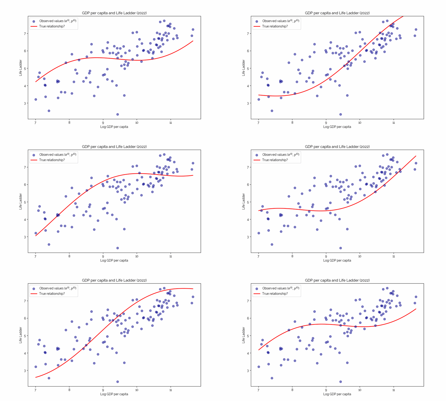
How do we decide on the best estimate $\hat{f}(\cdot)$ of the true relationship?
Loss functions
Our goal is to choose $\hat{f}(\cdot)$ such that, on average, our predictions are close to the true values… but what does this mean precisely?
Consider $y^{(i)} - \hat{f}(\mathbf{x}^{(i)}) = y^{(i)} - \hat{y}^{(i)}$, our prediction error, i.e., the difference between the true value and our predicted value. If this quantity is positive, we are underpredicting. If it is negative, we are overpredicting.
Intuitively, the closer the prediction error is to zero, the better our prediction. Let us formalize this…
Loss functions
- We denote our loss function as $\ell : \mathcal{Y} \times \mathcal{Y} \to \mathbb{R}$
- Intuitively, the loss function takes two inputs: the predicted value, and the true value and it outputs a number representing how different the two values are.
- For now, we assume our loss to be nonnegative, i.e., $\ell(\hat{y}^{(i)}, y^{(i)}) \geq 0$.
- We will also start by designing our loss function to be zero if and only if its two inputs are equal, i.e. $$\ell(\hat{y}^{(i)}, y^{(i)}) = 0 \iff \hat{y}^{(i)} = y^{(i)}$$
Loss functions
There are many different loss functions, each with advantages and disadvantages depending on the task, e.g.,
- Absolute loss: $\ell_\text{abs}(y, \hat{y}) = \vert\hat{y}-y\vert$
- Squared loss: $\ell_\text{sq}(y, \hat{y}) = \left(\hat{y} -y\right)^2$
- 0-1 loss: $\ell_\text{0-1}(y, \hat{y}) = \begin{cases}0 \text{ if } \hat{y} = y \\ 1 \text{ otherwise.}\end{cases}$
Empirical Risk Minimization
- Equipped with our loss function $\ell$, let us now reconsider the problem of choosing the best predictor $\hat{f}(\cdot)$.
- Suppose we have a set of predictors from which we can choose. We call this set the hypothesis class and denote it by $\mathcal{H}$.
- For instance, in the crop yield example, $\mathcal{H} = \{f_1, f_2, f_3\}$.
Empirical Risk Minimization
We want to find a predictor $\hat{f}(\cdot)$ which minimizes the so-called expected loss or population risk: $$L(f) := \mathbb{E}[\ell(y, f(\mathbf{x}))]$$
… unfortunately, this quantity is unobservable, so we cannot find its minimizer!
Empirical Risk Minimization
While we cannot compute the population risk, we can compute the so-called empirical risk or empirical loss, i.e., the average loss over the data set: $$\hat{L}(f) := \frac{1}{n}\sum_{i=1}^n \ell(y^{(i)}, f(\mathbf{x}^{(i)})).$$
Empirical risk minimization is the fundamental principle of choosing our predictor $\hat{f}$ such that $\hat{L}$ is minimized, i.e., $$\hat{f} = \underset{f \in \mathcal{H}}{\arg\min} \ \hat{L}(f) = \underset{f\in\mathcal{H}}{\arg\min} \ \frac{1}{n}\sum_{i=1}^n \ell(y^{(i)}, f(\mathbf{x}^{(i)}))$$
References
- James, G., Witten, D., Hastie, T., Tibshirani, R. & Taylor, J. (2021). An Introduction to Statistical Learning with Applications in Python (2nd Ed.). Springer.
- Mitchell, T. (1997). Machine Learning. McGraw Hill.
- Shalev-Shwartz, S. & Ben-David, S. (2014). Understanding Machine Learning: From Theory to Algorithms. Cambridge University Press.